Reparation and calibration of the torque sensor .

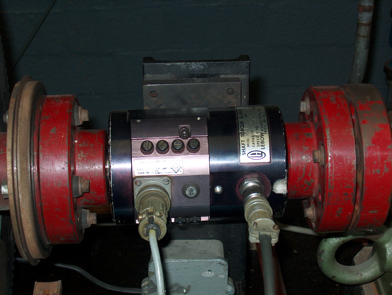
The torque is measured by a torque sensor , in our case the Lebow 1104-1K. This sensor is at 1 side connected to the crank-shaft of the engine and at the other side to a Foucault-brake which dissipates the power generated by the engine . The max RPM that this sensor can handle is 9000 RPM (this equals 9000/60 Hz = 150 Hz) , which is more then enough , since tests on the engine are only performed between 600 RPM and 1400 RPM (this equals 1400/60 Hz = 23,3 Hz) . The maximum torque this sensor can handle is 112,7 Nm . This is also more then enough , since the maximum torque that the engine can deliver is 40,7 Nm (at 1200 RPM) . Once one tries to perform tests at a number of revolutions higher then 1800 RPM , the whole installation shuts down automatically to protect the engine . Internally , trailing rings are attached around the bar that connects the crank-shaft and the brake . These trailing rings make contact with carbon bristles which ensure the electric contact and provide an analog output signal under the form of a tension . On the bar , strain gages are attached which are placed under an angle of 45 º and which are included in a Wheatstone bridge . When the engine is loaded , the bar will be submit to torsion . This way , there is no longer an equilibrium in the bridge and an electric tension , proportional to the torsion of the bar and thus to the torque generated by the engine is generated . This signal is sent to an amplifier , in our case the Daytronic 3278 . This amplifier converts the signal , received from the torque sensor , from a tension immediately into the value of the torque generated by the engine . This value is shown on a display . This device also possesses a ground and 2 different analog voltage outputs , which are proportional to the signal received from the torque sensor . One output is filtered between 0 Hz (DC) and 2 Hz , the other one between 0 Hz and 400 Hz . Both outputs have an accuracy of 0,05 % . The output voltage can vary from 0 V to +/- 5 V , which is ideal for us since the microcontroller we use , requires analog inputs between 0 V and 5 V and since no negative torques can be generated (the engine cannot be driven on by the brake) , we don’t need the negative voltage values . In case a negative value is obtained anyway , this can be considered as an incorrect measurement . The amplifier can handle an overrange of 50 % , but we stay below 40 Nm , so this is more then satisfying for our application .

To get our voltage input for the microcontroller , we decided to use the output signal from the amplifier . To be able to use this signal , the torque sensor had to be repaired and the amplifier had to be calibrated . Making a choice between the 2 available output signals of the amplifier , was very easy . Since the output with the 0 Hz to 2 Hz filter is provided for static measurements and that we worked dynamically , i.e. when the engine turns , we had no other choice than using the output signal with the 0 Hz to 400 Hz filter . We did make a connection for the 0 Hz to 2 Hz output signal as well , in case someone would need it one day .

Reparation of the torque sensor .

The torque sensor

In order to perform the calibration , we pinned the torque sensor in a lathe . This was done with enough precision , because when the sensor is pinned in too hard or to soft , the bar is submitted not only to tension , but to bending as well and then the output isn’t correct anymore . When this was done , we connected the analog output of the amplifier to a multimeter in order to be able to measure the generated tensions . When we moved the housing of the sensor a little , we noticed that the output wasn’t stable and we concluded that the sensor was defect so we had to repair it first .

In an effort to repair the sensor , following measures were taken :

• We removed the housing of the sensor and noticed that the bearings were defect , so we replaced them by new ones .

• We also noticed that the surfaces of the trailing rings weren’t worn out homogeneously , so we polished them .

• Also 2 carbon bristles were broken , so we replaced those as well .

• We checked the connection cable between the sensor and the amplifier and noticed that there was a bad contact , so we replaced all the contacts .

After these actions were done , the output signal was a lot more stable and we were able to start with the calibration of the amplifier .

Calibration of the amplifier .

The amplifier

Since the system had never been calibrated before , we had to find the correlation between the output voltage of the amplifier and the torque , generated by the engine , ourselves . This was done by loading the torque sensor with a dead weight , the procedure for this method is described in the manual of the torque sensor . Other procedures are possible , but we choose this one . The principle is very easy : a well known dead weight is hung up at a certain distance from the sensor , then the value on the display is set equal to the known torque and the output voltage is measured . For this method to be correct , it is necessary to load the sensor with a torque higher than the full scale and in positive direction . When we started with the calibration , we noticed that it was impossible to calibrate the amplifier , such as described in the manual . We suppose there must have been a defect since the amplifier went in overload without even being loaded . Luckily , another identical amplifier , which nobody used anymore , was available in the labo . With this amplifier , we were able to perform the calibration correctly . Once the amplifier was calibrated , we put several loads on the sensor to check if the relation between the torque and the output voltage is linear . Via linear regression , the eventual multiplication factor is then found .   

The maximum torque the sensor can handle is 112,7 Nm . Thus the minimum load that must be applied to calibrate the sensor is 56,35 Nm . For our measurements , we used several weights , which we weighed in the labo of the “Burgerlijke Bouwkunde” with a very accurate balance . To be able to hang up the weights , we used a steel bar and a hanger which was placed at exactly 1 meter from the sensor to simplify the calculations afterwards . When a bigger load is hung at the sensor , the bar bends more . For correct measurements , the bar must be water-leveled every time , which we ensured by shoving a conical pin further and further under the bench-clamp which held the sensor at increasing loads .

To calculate the contribution of the bar to the total torque , we modeled it as a divided load . The mass of the bar is 2,984 kg and its length is 1,501 m .

The mass per length is then : a = 1,98 kg/m .

The torque of the bar , which is always present , is then :

                     l-ε

C_bar = g * ∫      a * x * dx = g * a * ( l²  - 2 * ε * l )

                     -ε

where : a = 1,98 m

             g = 9,81 m/s²           

             l = 1,501 m

             ε = 0,088 m 

ε is the part of the bar that hangs on the other side of the sensor then the one where the actual load is hung up  . By expressing the integral as above , the contribution of this part disappears with an equivalent contribution on the other end .

This results in :   C_bar = 19,3 Nm .

The hanger weighs 0,.39922 kg . At a distance of 1 m , it gives following contribution to the total torque :

C_hanger   = 0,39922 * 9,81 * 1 = 3,91 Nm

To make it possible to load the sensor with different weights , we disposed of 5 different masses :

For the actual calibration , we used mass number 5 . Together with the bar and the holder , this gives a torque of 76,84 Nm . We calibrated the amplifier by hanging this load at the sensor and tuning the amplifier until this value was written on the display .

The next step , was to hang different loads at the sensor to find the correlation between the output voltage of the amplifier and the torque . This gave following results :

In this table B stands for “bar” and H stands for “holder” . 

After linear interpolation , we get following relation between the torque and the output voltage :

Torque = 20,02 * Voltage – 1,11 * 10^-2

We simplified this relation into :

Torque = 20 * Voltage

The covariance for the linear interpolation is = 68,84 .