• Hardware
  1. Electrical schemes
  2. Printed Circuit Boards
  3. Body design
• Software
• Errors

Software

The program for controlling the robot was written in assembler for the PIC microcontroller. It was written and compiled with the program MPLAB and simulated with the program PIC Simulator IDE.

The source code of the program can be found here.

1. Main flowchart of the program

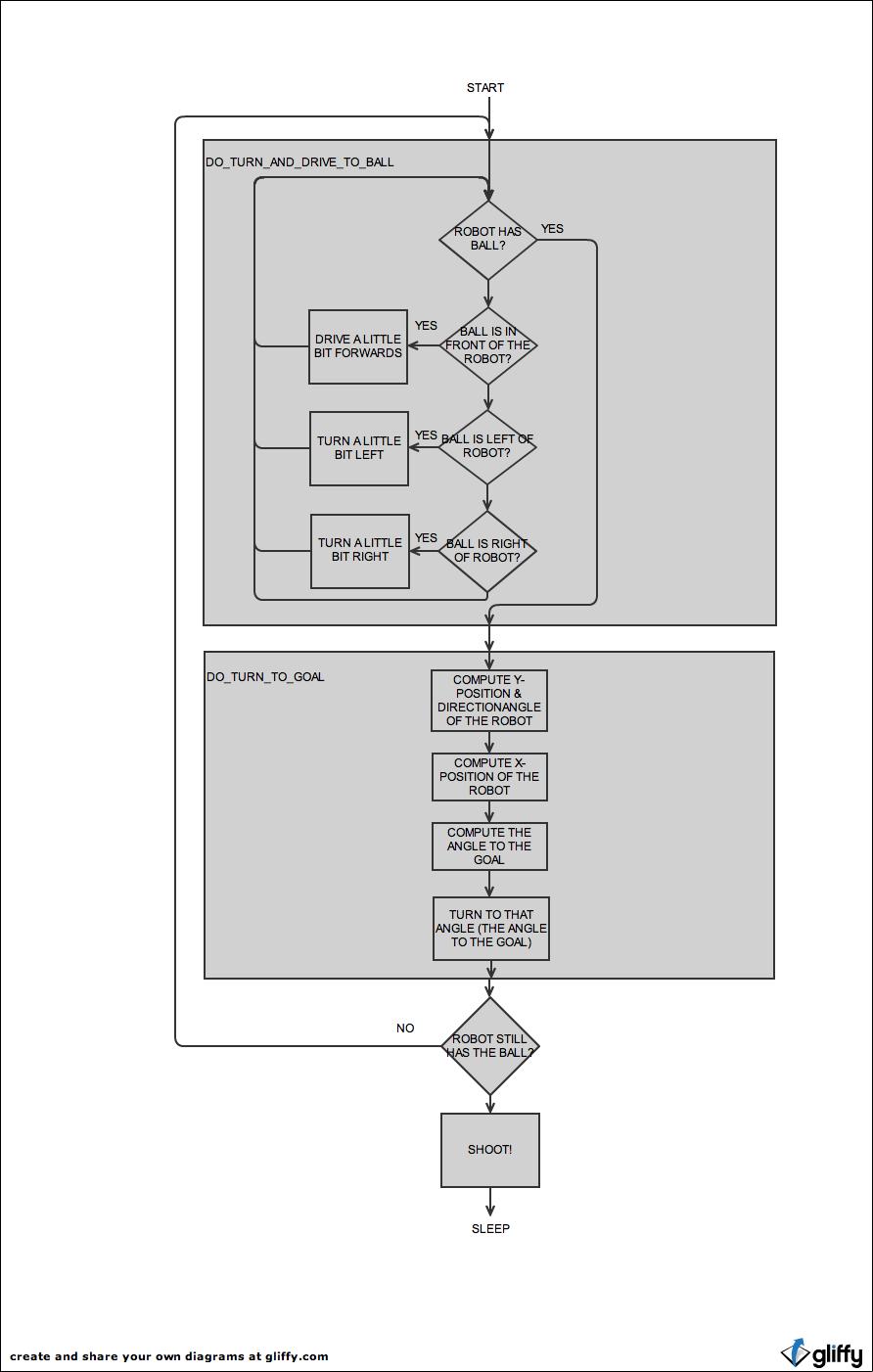
The first important routine that the robot will use, is DO_TURN_AND_DRIVE_TO_BALL. When the robot is in the routine, he will eventually be pointing towards the ball (after multiple axial right/left turns) and he will drive towards the ball until the IR distance sensor at the front reaches 4V (the routine GET_BALLDETECTIONBOOLEAN checks if this is the case, every time we cycle through DO_TURN_AND_DRIVE_TO_BALL; and we cycle through this routine until we arrive at the point where the routine GET_BALLDETECTIONBOOLEAN will set a flag high, to signal that fact where the robot has possession of the ball).

The, the second important routine that the robot will use, is DO_TURN_TO_GOAL. There, multiple subroutines will be called in order to compute the Y-position of the robot - which is the average value of the 3 greysensors beneath the robot, to compute the directionangle of the robot - which is again based on the 3 greysensors (please note: for the mathematical calculations, we used open source routines; source: http://avtanski.net/projects/math), and to compute the X-position. However, to compute the X-position, it would be inaccurate to rely on one sharp distancesensor at the right side of the robot, even when that sensor is not perpendicular to the sidewalls: the risk of measuring a distance which outside the range of the sensor would be too high. Therefore, calculating the X-position is done by aligning the robot with the sidewalls in order to have the sharp distancesensor perpendicular to the sidewalls. Then, if the robot knows his Y-postion and his X-position, he is aware of his position on the field, and he can decide how to turn towards the goal.

However, chances are high that the robot will have lost the ball by the time that he will be pointing towards the goal (after all, the movement to align the robot with the sidewall will most probably result in a loss of the ball): therefore, the main routine will check if the robot still has the ball (by calling GET_BALLDETECTIONBOOLEAN, and by checking the flag that is manipulated by GET_BALLDETECTIONBOOLEAN): in case he has lost the ball, the whole program will start again...

At a certain moment, we considered to use omnidirectional wheels / meccanum wheels. Using such wheels would allow the robot to position itself optimally towards the goal, by driving around the ball. Now, chances are very high that the robot will lose the ball as soon as he positions himself towards the goal (or even sooner: when he aligns himself with the sidewalls, in order to compute his X-position).

top

2. Important subroutines

Next, we will discuss some of the more advanced subroutines:

1. Computation of the orientation of the robot: COMPUTE_CURRENT_DIRECTIONANGLE_2
2. Computation of the angle to the goal: COMPUTE_ANGLE_TO_GOAL

2.1 Computation of the orientation of the robot: COMPUTE_CURRENT_DIRECTIONANGLE_2

Because the robot has to make an angle to kick the ball into the goal, it needs to be able to determine its orientation on the field. This is possible by use of the greyscale which covers the whole surface of the field.

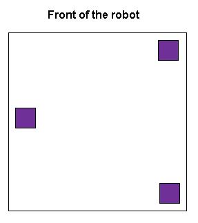
With 3 greyscale sensors, placed in a triangular configuration, it is possible to determine the full (360°) orientation of the robot on the field. The position of the greysensors under our robot can be seen in following figure (top view):

Next we have to define a reference direction from which the angle is measured:

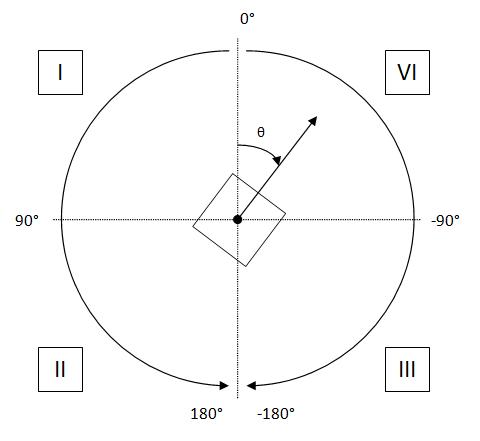
We defined 0° to be the vertical alignement of the robot in the direction of the opponents goal. The calculation of the angle will depend on the quadrant the robot is oriented into.

We used an 8 bit register to store the angle into, we defined it like in the table below:

After we defined these arrangements, the calculation of the angle can be considered:

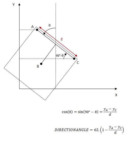
This figure represents the position of the greyscale sensors on the field if the robot makes a certain angle with the vertical alignement.

The 2 greyscale sensors at the side of the robot (A and C) are separated by a fixed distance d. They produce a signal in function of the vertical (y-) position of the robot on the field.

So, with these 3 values we can calculate the cosine of the orientation-angle, and by taking the 1st order Taylor-series of the arccosine, and accounting our angle definition, we become an approximation of this angle.

This formula applies for the first quadrant, and by an analogue way, we can determine the formulas for the other quadrants.

Eventually, we become a decision tree, which is easily translated into assembler code:

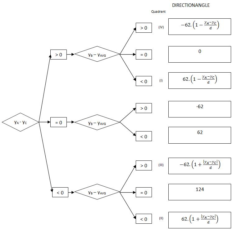
The problem with these formulas is that there is a devision of two numbers of about the same size: this can be avoided by rearranging the calculation order (see source code comment).

top

2.2 Computation of the angle to the goal: COMPUTE_ANGLE_TO_GOAL

The angle the robot has to have to be oriented towards the opponents goal, is a function of the robot x- and y- coordinates on the field.

This can be seen on following figure:

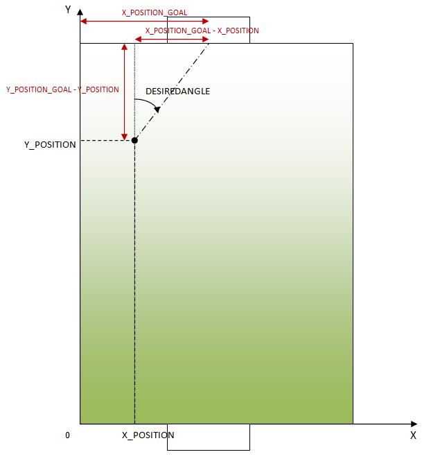
Now, the angle can be approximated by the arctangent:

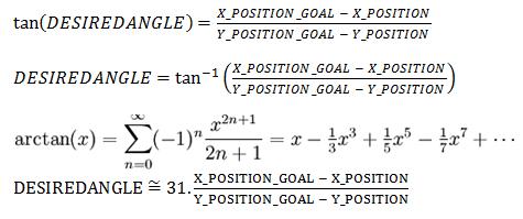
Here again we accounted our angle definition with the factor 31: for example, if the angle is 45° then the tangent will be 1, and hence the fraction detaX/deltaY will be one, so the desired angle is 31, which equals 45°.

top