Importance of the software
A good robot has sensitive but robust sensors and actuators, a good mechanical design and high reliability. However, none of these characteristics will have any effect if the controller software does not function well. It is the responsibility of the microcontroller to read the sensors and act on the readings in an intelligent manner. Imagine a soccer-playing robot that thinks the sun is the infrared-ball and constantly tries to kick the sun towards the goal…
The boundary conditions
The assignment proposed a PIC-microcontroller being used to control the robot’s movements. Specifically, a choice still had to be made between a PIC16F876 and a PIC16F877 microcontroller. These 2 versions of the same controller only differ in that the latter has more analog input possibilities (and is also able to communicate with other microcontrollers, but that was not an interesting feature for our purposes, since we wouldn’t need that much calculative power). We decided to go for the (slightly more expensive) PIC16F877, because we would rather be confronted with a surplus of input capacity than with a shortage of it. (If you are interested in the possibilities of this microcontroller, search the internet for “datasheet PIC16F877”.)The PIC-microcontroller came with the so-called PIC-kit, a USB-adaptable code input device for the microcontroller. You just have to provide a .hex-version of the programme code (which we obtained with software called MPASM) and then input it into the microcontroller via the PIC-kit interface. Very practical!
Obviously, the programme could in theory be written in any higher programming language. C or Basic would have seemed obvious choices. However, our professor specifically asked us to write the code directly in Assembler (the reason being that this would guarantee a faster execution of the programme). The PIC16F87X-series has a “special” limited instruction set: it consists out of only 35 instructions! This is as much an advantage as it is a disadvantage: for example, there is no instruction for multiplication – you have to write it yourself, using the 35 instructions that are available.
Sensors/actuators
The programme needs to read all of the sensors and drive all of the actuators. The sensor array consists out of 3 grey-value sensors, 2 SHARP (IR) distance measuring devices, 1 PING)))-sonar distance measuring device and 3 values coming from IR-sensors placed on the exterior of the robot (see below), meant for localization of the ball. The actuation is done by 3 electric drives (brushless DC motors), of which 2 are controlled with PWM-method and the third just by digital output (0 for standstill and 1 for all-out – this is the motor for the dribbler device). For more information, see the section about the sensors.
The above mentioned IR-sensors which are used to localize the ball, are distributed along the exterior of the robot as can be seen on the figure below.

From the comparison of, respectively, A & B (the couple (1))and D & C (the couple (2)), we can learn whether the ball is left (A>B and/or D>C) or right (B>A and/or C>D) of the robot. To know if the robot is roughly “in front of” or “behind” the robot, we use the sum of A & B and compare this sum with a calibrated reference: from tests, we know how much A + B has to be for the ball to be in front of the robot.
Outline of the programme
Obviously, before you can score a goal, you have to gain possession of the ball. In order to do this, you first need to localize the ball, then turn towards it and close in on it, then grab it. Next, you need to turn towards the goal, then drive the ball into the goal. The following flow chart describes graphically what I just explained.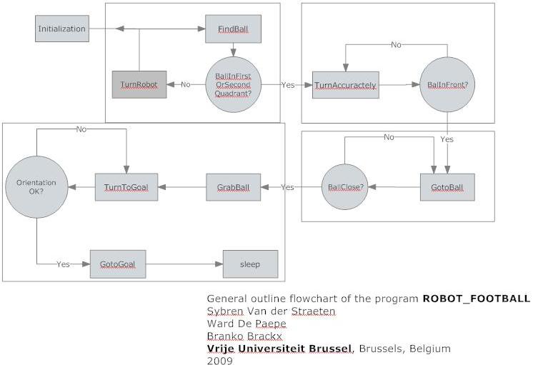
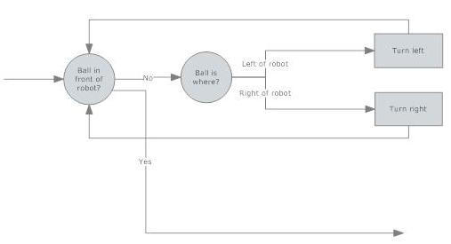
First, we will turn the robot until it roughly faces the ball; the criterion here is (3). As long as (3) is smaller than the reference value, we will turn either right or left, depending on (2). This algorithm is presented graphically below.
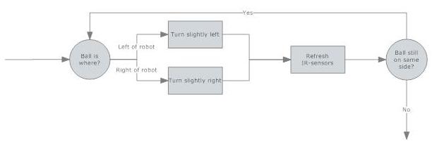
Next, we will turn the ball more accurately until the ball is exactly in front of the robot. The criterion here is (1): if during the “previous iteration” the ball was left of the robot, and during the “present iteration” the ball is right of the robot (i.e. the value of (1) changed, compared to the previous iteration), we are sure that the ball was just in front of the robot – within the tolerance, provided by the angle by which you turn the robot during every new iteration. For example: the ball is at 7° left of the robot. We turn the robot right by 5°. The ball is still left of the robot (now by 2°), so we turn once again. The ball is now right of the robot by 3°, and we stop the turning. The tolerance here is 5°: if the ball was 0,0000…1° left of the robot and we turn once more, it is now at 4,99……°(right). Needless to say, if you make the robot turn in smaller steps, you will have more accuracy in getting the ball in front of the robot. However, this accuracy is severely limited by that of your sensors: if you can only determine where the ball is within a tolerance of 10°, it makes no sense of taking turning steps of 2°… For our sensors, this limitation turned out to be quite restrictive: we were happy to obtain a practical tolerance smaller than 15°! Again, the following graph might make it easier to understand this sub-algorithm.
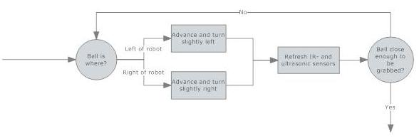
Now that we’re sure that the ball is dead ahead, getting close enough to grab seems pretty straightforward. To be sure we don’t miss the ball, we will constantly keep turning towards it, this time with as small a tolerance as our sensors permit us. See the chart below…
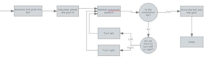
Finally, all that is left is to grab the ball (done by turning the dribbler on and advancing rather quickly towards the ball, so that the dribbler “slides” over the ball), turn towards the goal (done by calculating where the goal is and then turning until the actual orientation corresponds to the calculated one) and drive the ball into the goal. For the last time, a flow chart…
That’s it, we scored!
Of course, now that we have devised a strategy on how to score, we need to translate this “pseudo-code” to actual code. Before trying the actual code on the robot, I tested all of it on a simulator programme (a programme that lets you follow the execution of your code, line by line, and shows you the contents of every memory register, every step of the way) called PIC Simulator IDE (trial version) until all obvious bugs had been removed.
Source code
A disadvantage of programming straight in Assembler is that the final programme is a giant heap of code (about 1600 lines). I spent a lot of time making the programme as modular as possible, but there is also a drawback to this: the controller has a return stack of only 8 addresses! So, at all times, one has to be put attention into not calling too many subroutines.The source code is best opened with Notepad++ (for lay-out reasons). The starting point for reading the programme is probably “LOOP_Main”. Following all calls will take you through the programme as I explained it above.
Download the source here
Copyright © 2009 • Ward De Paepe • All Rights Reserved |